9/1/2022 (First Posted)
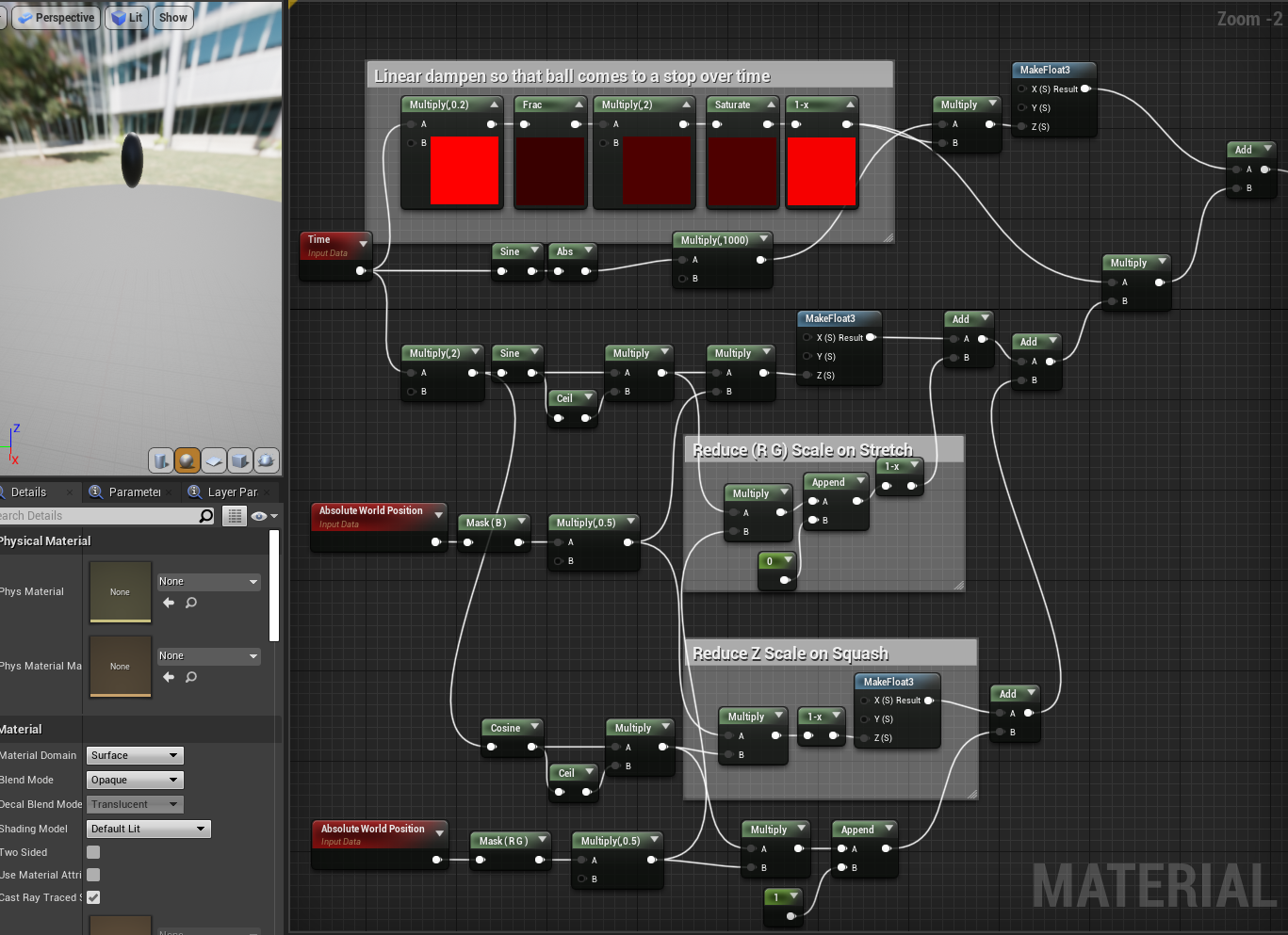
This is what I’ve been exploring the past month with (Principal Tech Artist at Polyarc) Tyler’s help! Always wanted to try creating sand-like rippling trails, so I’m really happy to get something like that working. I’m using blueprints for the propagation, so the next step is exploring Niagara more and relying less on CPU.
- Using a material to animate a bouncing ball with squash and stretch.
- Niagara to apply horizontal force and duplicate the balls.
- Color atlas and curves to change the colors and shade the ground ripples.
- Render target that draws relative to mouse position and mouse click, and creates ripples in the ground with vertex offset.
This post will guide you through my process of creating the base shader, step by step, through the eyes of someone who is 100% new to shaders.
Starting with the Basics:
Coming from nearly zero shader experience, getting a grasp of the basics is essential!
Some of the nodes have similar names to processes in other programs. For example there’s a multiply node and saturate node in Unreal Engine. Do not be fooled by the names! They are different things and it will only confuse you to make those incorrect connections.
Helpful tips:
- If you’ve fiddled around with the contrast curve graph in Photoshop or animation time graphs, shaders are a lot like that – it involves lots of graph visualization.
- Also I recommend thinking in terms of 0-1.
- Black represents a value of 0 or lower, while white (think of a light switched “on”) represents a value of 1 or higher. Higher than 1, and the white will go into emissive values.
- Shaders use interpolated colors to represent coordinates and positions in space. The blending of colors in UE is done with additive colors (CMYK!!)
- This is super confusing because although letters of RGBA are referenced as directions, the blending itself is additive. So rather than thinking of painting with paints, think of overlaying colored lights.
Enough talk, it’s easier to explain things with some visual guides.
Time
For reliable animation/change
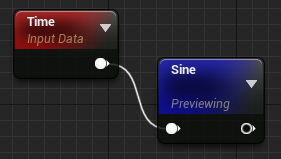
How to understand this?
We can use a handy dandy graph.
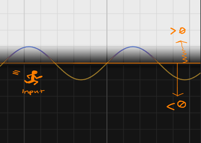
Forget about time for a second, this is a sine with an input of x. Meaning, the input is just the value along the x axis here, and then plotting a point. Joining to form this yellow squiggly.
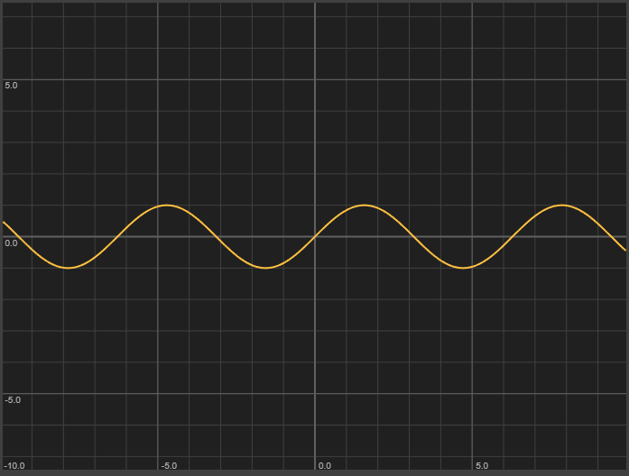
So now if we consider how time works…. 1, 2, 3, 4, 5…at a constant rate.
We can visualize our shader traveling along the x axis of this squiggly at the rate of time.
If you can understand this, it’s already a huge step.
Since 0 in shaders is represented as black, and 1 is white, we wanna keep this in mind when working with shaders to keep our values easy to control and clean. The nice thing about sine here is that the highest value is 1 and it swings back to -1.
We send our little running man along the x axis to draw the path and track the output values.
Constant Bias Scale
To bring all values up to the range between 0 and 1 we can apply a constant bias scale node. This node does an operation of adding a number, and then scaling by a number. In this case we use the default of adding 1 and scaling by 50% or half.
Adding and Subtracting
Adding or subtracting is simple enough to visualize on a graph. You simply move a point up or down since going up will bring you to higher values and going down will take you to lower values.
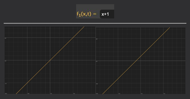
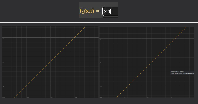
So if we wanna move the sine wave up into the gradient above 0, we can just add 1. Now the sine will have a low value of 0 and a high value of 2:
Dividing/Multiplying in terms of basic Scaling
This was definitely more difficult for me to wrap my head around. The trick is to realize that the center pivot of all scaling operations is along the x axis.
Additionally if you scale the output value, it’ll scale along the y axis. Think of dragging the transform box in photoshop, and in addition its pivot is at 0 on the y axis.
Adding one to the sine operation:
Dividing (Scaling) along the y axis with pivot point of x axis:
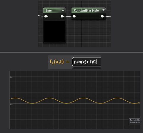
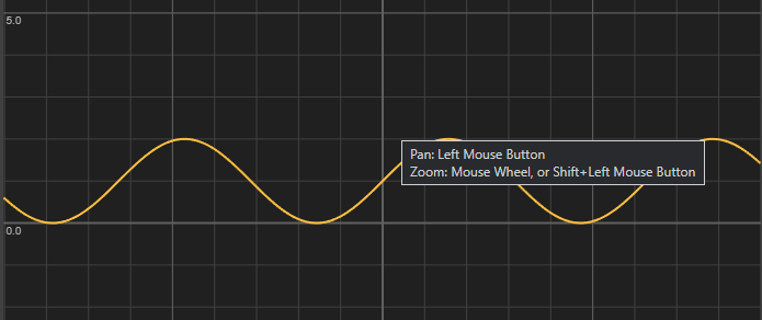
So now we see this in the preview:
(sin(x)+1)/2
Before:

sin(x)
The difference is difficult to notice, but in the new preview the color stays black for a much smaller duration. This is because the values aren’t dipping less than 0, into the negatives.
Abs
Once you understand this basic process of graph manipulation, it’s easy to apply this way of thinking to different types of graphs and mathematical operations.
For the bouncing ball I went with an abs value of sin graph, since it resembles the motion of…a bouncing ball. It also keeps the values nicely between 0 and 1 without much extra work.


Visualized in the preview, the material looks like this:
Remember, 0 is black and 1 is white 👍
Vertex offset
Now it’s time to make this move!
We can easily do this by taking this output and applying it to all vertices in the up direction.

When applying offsets and trying to manipulate position, it helps to make a switch in your mind from graph mode to vector math mode.
So we convert this 0-1 float value to a vector 3. We only wanna change the up vector strength. So now we go from (0,0,0) to (0,0,1). The world position offset adds the result to the world position offset regardless of what node you feed into it.


Multiply/divide in terms of diminishing/emphasizing other parts of the shader (different perspective on scaling)
Earlier in this post multiplication was used to scale the output results for a function. The second way to use multiplication is straightforward – to increase or decrease as a multiplier.


Adding squash, stretch, making the ball gradually bounce less

If we take the same output from before and apply it directly into the world position offset output, it’s going to offset the vertices based on world position. It won’t be a uniform scaling as you may expect. Going from (0,0,0) to (1,1,1)

Instead, if we only isolate the Y direction of the vector and apply our output to that, there shouldn’t be any issues:

(Emission here gets higher as we get to higher values at the top. There are values going below zero near the bottom, although visually it is all a uniform black. Confusing, I know.)
An important note is that once we mask R,G,B, or A values, we also change the data structure (?) Only masking in the B (Up Vector) means that we only receive the float value.


So now, we want to apply this to the bouncing animation timeline to make this ball stretch when it bounces up.
Using the multiplier here to scale the lower values lower and higher values higher and adding these changes to the bounce, we can control the stretch.
Now the challenge is in timing the stretch.

We can add another multiply node scaling based on the abs value. When multiplied by 0, the value will return 0, while 1 will be its max scale.

This shows us what the stretch looks like on its own.

If we reconnect the base bouncing animation…
.
The stretch will be fully active at the top of the bounce, and not active at the bottom of the animation.
What we want to do is:
- Decrease the animation time of the stretch (make it more sudden)
- Make the timing adjustable

We want the stretch to look something like this

Using our handy shaping functions an idea comes through.
All about shaping functions here: https://thebookofshaders.com/05/


This is another more precise method with a couple more steps (pun not intended):

Btw, we can disregard the PI division in unreal because the sine wave defaults to a rational number.
Finally, balls don’t bounce infinitely, so let’s make this one come to a stop.

We do this by creating a frac and multiplying the inverse result with the output to dampen until it comes to 0.
For squash, I’ll do the same with both the forward and right channels (R,G)
Using cosine to offset the squash to be at max value at the low value of the abs sine.


Using an append node to add the vector 2 value with the vertical vector 3 value from earlier.
You may have noticed that the volume of this ball changes drastically when stretching and squashing. Let’s fix that first.